Confocal Paraboloidal Coordinates: Operators, Separation, and a Boundary-Value Problem

Abstract

We develop a self-contained account of confocal paraboloidal coordinates in the Moon–Spencer notation \((\mu,\nu,\lambda)\), with every formula checked symbolically against their Table 1.11 (2nd ed., pp. 44–46). The note covers the geometry and coverage of the coordinate surfaces, the scale factors and vector operators (including a correction to the printed Laplacian prefactor on p. 45), separation of Laplace’s equation with Moon and Spencer’s constants \(\alpha_2,\alpha_3\), an algebraic extension to the Helmholtz equation, and the elementary Dirichlet problem between two confocal elliptic-paraboloid electrodes, with an exact log solution and a computed field plot. Differences from the Morse–Feshbach presentation on pp. 664–665 are flagged in the text.

Laplace’s and Helmholtz’s equations separate in only a handful of three-dimensional orthogonal coordinate systems; the most general families are the confocal ellipsoidal coordinates and their limiting case, the confocal paraboloidal coordinates [1, 2]. In the latter, two families of coordinate surfaces are elliptic paraboloids opening in opposite directions and the third consists of hyperbolic paraboloids, so the system is the natural one for fields near paraboloidal conductors, reflectors and saddle-shaped boundaries [5]. Unlike parabolic-cylinder or rotational parabolic coordinates, the system has no translational or rotational symmetry, and the three separated equations are coupled through two common separation constants, which makes the eigenvalue problems genuinely three-dimensional.

The coordinates are tabulated in the handbook of Moon and Spencer [1], whose notation \((\mu,\nu,\lambda)\) we adopt; a number of the elementary separated solutions printed there were later corrected [3]. Our aim is a compact, self-contained account for physicists: the definition and geometry including coverage and degenerate surfaces (Sec. 2), the vector operators (Sec. 3), separation of the Laplace and Helmholtz equations (Sec. 4), and an elementary boundary-value problem (Sec. 5). Every formula has been checked symbolically.

2 Coordinates

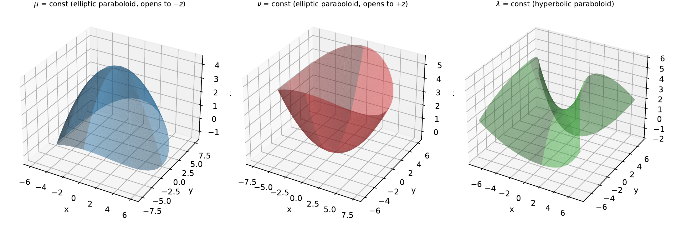
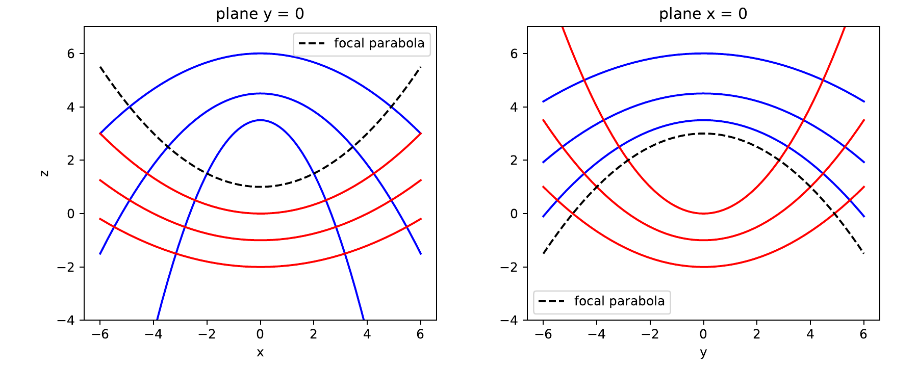
Following Moon and Spencer [1, Table 1.11], let \(b>c>0\) and \((u^1,u^2,u^3)=(\mu,\nu,\lambda)\) with \(\infty>\mu>b>\lambda>c>\nu>0\).¹ Then \[\begin{equation} x^2=\frac{4(\mu-b)(b-\nu)(b-\lambda)}{b-c},\qquad y^2=\frac{4(\mu-c)(c-\nu)(\lambda-c)}{b-c},\qquad z=\mu+\nu+\lambda-b-c . \end{equation}\] The three coordinates are the roots \(\sigma\) of \(\frac{x^2}{b-\sigma}+\frac{y^2}{c-\sigma}=4(z-\sigma)\), giving \[\begin{align} \mu&:\ \tfrac{x^2}{\mu-b}+\tfrac{y^2}{\mu-c}=-4(z-\mu), & \nu&:\ \tfrac{x^2}{b-\nu}+\tfrac{y^2}{c-\nu}=4(z-\nu), & \lambda&:\ \tfrac{x^2}{b-\lambda}-\tfrac{y^2}{\lambda-c}=4(z-\lambda), \end{align}\] i.e. elliptic paraboloids² opening towards \(-z\) and \(+z\), and hyperbolic paraboloids (Fig. 1). Since only \(x^2,y^2\) are determined, each triple \((\mu,\nu,\lambda)\) labels four points \((\pm x,\pm y,z)\). The planes \(x=0\) and \(y=0\) are where \(\mu\) or \(\lambda\) reaches \(b\), respectively \(\lambda\) or \(\nu\) reaches \(c\). The focal parabolas are \(x=0,\ y^2=-4(b-c)(z-b)\) (\(\lambda=\mu=b\)) and \(y=0,\ x^2=4(b-c)(z-c)\) (\(\lambda=\nu=c\)), Fig. 2.

3 Scale factors and vector operators

\[\begin{equation} h_\mu^2=\frac{(\mu-\nu)(\mu-\lambda)}{(\mu-b)(\mu-c)},\quad h_\nu^2=\frac{(\mu-\nu)(\lambda-\nu)}{(b-\nu)(c-\nu)},\quad h_\lambda^2=\frac{(\lambda-\nu)(\mu-\lambda)}{(b-\lambda)(\lambda-c)} . \end{equation}\] In the Morse–Feshbach coordinates \(\xi_n=\sqrt{2\sigma_n}\) (footnote in Sec. 2) the scale factors carry the Jacobian \(d\sigma/d\xi=\xi\), \(h_{\xi_n}=\xi_n h_{\sigma_n}\), e.g. \(h_1=\xi_1\big[(\xi_2^2-\xi_1^2)(\xi_3^2-\xi_1^2)/((\xi_1^2-a^2)(\xi_1^2-b^2))\big]^{1/2}\) [2, p. 664]. The Laplacian there takes the form \(\sum_n h_n^{-2}f_n^{-1}\partial_{\xi_n}(f_n\partial_{\xi_n})\) with \(f_n=\xi_n^{-1}\sqrt{(\xi_n^2-a^2)(\xi_n^2-b^2)}\), equivalent to our \(w_s\), and the singular points sit at \(\xi=0,\pm a,\pm b\) instead of \(s=b,c\). With \(H=h_\mu h_\nu h_\lambda\) and unit vectors \(\mathbf e_q=h_q^{-1}\partial_q\mathbf r\), the triad \((\mathbf e_\mu,\mathbf e_\lambda,\mathbf e_\nu)\) is right-handed for \(xy>0\).³ Then \[\begin{gather} \nabla f=\sum_q \frac{\mathbf e_q}{h_q}\partial_q f,\qquad \nabla\cdot\mathbf F=\frac1H\sum_q\partial_q\!\Big(\frac{H}{h_q}F_q\Big),\\ (\nabla\times\mathbf F)_{q_1}=\frac{1}{h_{q_2}h_{q_3}}\big[\partial_{q_2}(h_{q_3}F_{q_3})-\partial_{q_3}(h_{q_2}F_{q_2})\big], \quad (q_1,q_2,q_3)\ \text{cyclic in}\ (\mu,\lambda,\nu), \end{gather}\] \[\begin{equation} \nabla^2u=\sum_{s\in\{\mu,\nu,\lambda\}}\frac{(s-b)(s-c)\,\partial_s^2u+\tfrac12(2s-b-c)\,\partial_su}{\prod_{q\neq s}(s-q)} . \end{equation}\]

4 Separation

For \(\psi=M(\mu)N(\nu)\Lambda(\lambda)\), Laplace’s equation separates into the three equations printed by Moon and Spencer [1, Table 1.11, p. 46]: \[\begin{align} &(\mu-b)(\mu-c)M''+\tfrac12[2\mu-(b+c)]M'-[\alpha_2-\alpha_3\mu]M=0,\\ &(b-\nu)(c-\nu)N''+\tfrac12[2\nu-(b+c)]N'-[\alpha_2-\alpha_3\nu]N=0,\\ &(b-\lambda)(\lambda-c)\Lambda''-\tfrac12[2\lambda-(b+c)]\Lambda'+[\alpha_2-\alpha_3\lambda]\Lambda=0, \end{align}\] with separation constants \(\alpha_2,\alpha_3\). All three are the single equation \((s-b)(s-c)F''+\tfrac12(2s-b-c)F'+(\alpha_3 s-\alpha_2)F=0\) written on the three intervals; the \(\lambda\) equation is multiplied by \(-1\) so that its leading coefficient is positive.⁴

Helmholtz equation (our extension).

By the \(k=2\) identity, \((\nabla^2+k^2)\psi=0\) separates as well. Each printed equation acquires the term \(+k^2s^2F\) added to its \(-[\alpha_2-\alpha_3 s]F\) term (for \(\mu,\nu\)), and \(-k^2\lambda^2\Lambda\) for the \(\lambda\) equation: \[\begin{equation} (s-b)(s-c)F''+\tfrac12(2s-b-c)F'+(k^2s^2+\alpha_3 s-\alpha_2)F=0 . \end{equation}\] This form is derived here; we have not compared it with Moon and Spencer’s Helmholtz table.

5 Example: field between two confocal paraboloids

Take the region between the surfaces \(\mu=\mu_1\) and \(\mu=\mu_2\) (\(b<\mu_1<\mu_2\)), held at potentials \(V_1,V_2\). A solution depending on \(\mu\) alone (\(k=\alpha_2=\alpha_3=0\)) satisfies \(\big(\sqrt{(\mu-b)(\mu-c)}\,u'\big)'=0\), so \[\begin{equation} u=V_1+(V_2-V_1)\frac{G(\mu)-G(\mu_1)}{G(\mu_2)-G(\mu_1)},\qquad G(\mu)=\ln\!\big[2\mu-b-c+2\sqrt{\mu-b}\sqrt{\mu-c}\big], \end{equation}\] as printed in [1, p. 46]. The field is \(\mathbf E=-\mathbf e_\mu h_\mu^{-1}u'(\mu)\), with \(u'=(V_2-V_1)/\{[G(\mu_2)-G(\mu_1)]\sqrt{(\mu-b)(\mu-c)}\}\).⁵

Physical remarks.

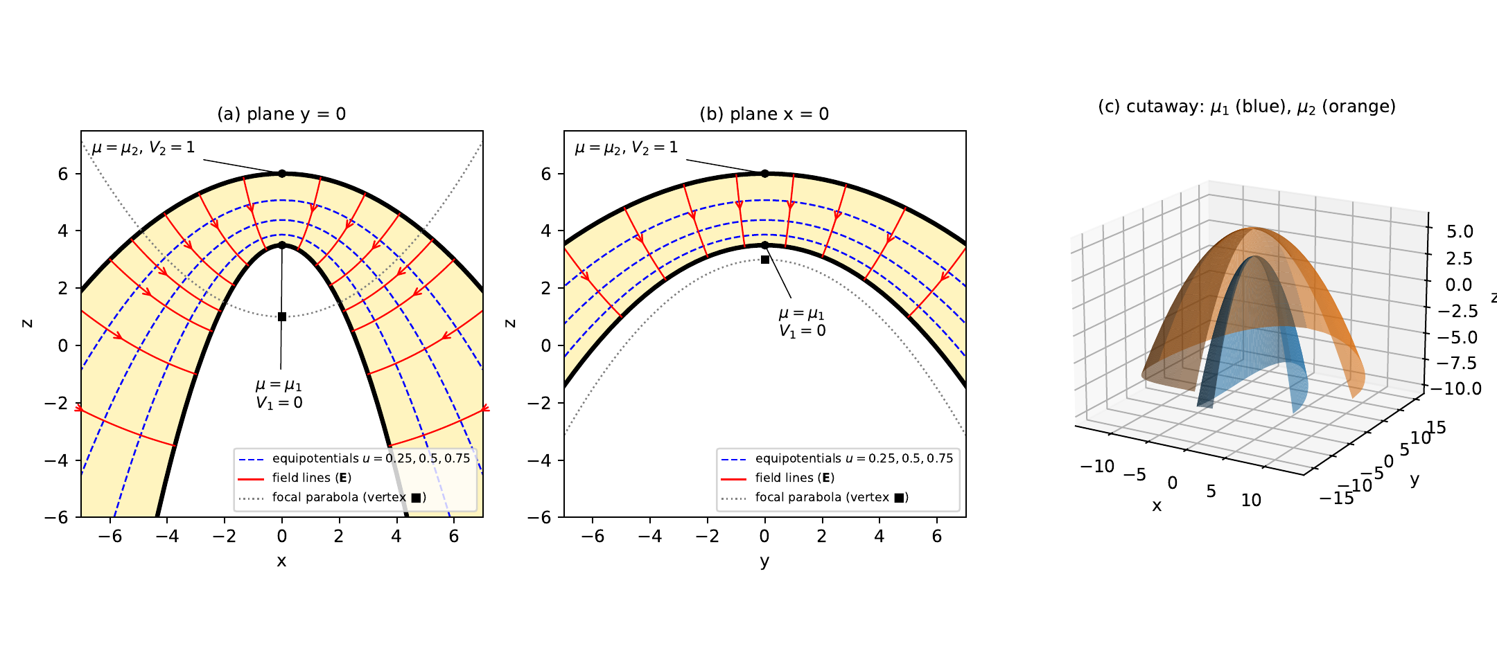
The equipotentials are the confocal paraboloids \(\mu=\text{const}\), and \(\mathbf E\) is everywhere normal to them. Its magnitude is \[\begin{equation} |\mathbf E|=\frac{|C_2|}{h_\mu\sqrt{(\mu-b)(\mu-c)}}=\frac{|C_2|}{\sqrt{(\mu-\nu)(\mu-\lambda)}},\qquad C_2=\frac{V_2-V_1}{G(\mu_2)-G(\mu_1)}, \end{equation}\] so on a given electrode \(\mu=\mu_i\) the field, and the surface charge density \(\varepsilon_0|\mathbf E|\), is largest where \((\mu_i-\nu)(\mu_i-\lambda)\) is smallest, i.e. near the vertex region, and it decreases as \(\nu\to-\infty\) along the surface. Because \(G\) grows only logarithmically, \(G\sim\ln(4\mu)\) for \(\mu\to\infty\), the potential difference between widely separated paraboloids grows slowly. The electrodes are unbounded, so total charge and capacitance must be defined per suitable truncation; we do not pursue that here. Since the region is unbounded, uniqueness of the Dirichlet problem also requires a condition at infinity.

6 Conclusion

Confocal paraboloidal coordinates \((\mu,\nu,\lambda)\), with Moon and Spencer’s ranges and scale factors, give an orthogonal system whose Laplacian separates with two shared constants \(\alpha_2,\alpha_3\). The printed operators on pp. 44–45 match the metric once the Laplacian prefactor is restored to the form implied by \(\nabla\cdot\nabla\); the separated Laplace equations and the \(\alpha_2=\alpha_3=0\) special solutions on p. 46 then follow and have been verified. The same identities extend separation to \((\nabla^2+k^2)\psi=0\), with an extra \(k^2s^2\) term in each ordinary differential equation. As a first application, the potential between two confocal electrodes \(\mu=\mu_{1,2}\) depends on \(\mu\) alone and is elementary; the field is normal to the electrodes and strongest near the vertices. Natural next steps, not treated here, are uniqueness conditions at infinity for unbounded electrodes, capacitance under truncation, Morse–Feshbach’s Stäckel data and separated forms, and the literature on paraboloidal wave functions for nonzero separation constants.

Acknowledgments

Drafting, symbolic checks (using sympy), and figures were prepared with the assistance of an AI tool. All results were verified by the author against Moon and Spencer and Morse and Feshbach.

References

Ranges, transformation and surfaces as printed in Table 1.11 of the 2nd edition, consulted via the author’s transcription; all were checked symbolically. The restriction \(\nu>0\) confines the system to the interior \(x^2/b+y^2/c<4z\) of the paraboloid \(\nu=0\). The formulas below remain valid for \(\nu<0\), which extends the coordinates to all of space; this extension is ours.↩︎
We follow Moon and Spencer [1]. Morse and Feshbach [2, Part I, p. 664, item XI] (cited here from a user-provided transcription of that page) use square-root coordinates \((\xi_1,\xi_2,\xi_3)\) and constants \(a>b\), with \(x^2=\prod_n(\xi_n^2-a^2)/(a^2-b^2)\), \(y^2=\prod_n(\xi_n^2-b^2)/(b^2-a^2)\), \(z=\tfrac12(\xi_1^2+\xi_2^2+\xi_3^2-a^2-b^2)\). These coincide with ours under \(\xi_1^2=2\mu\), \(\xi_2^2=2\lambda\), \(\xi_3^2=2\nu\), \(a^2=2b\), \(b_{\rm MF}^2=2c\). The \(z\) axis is the same, with no sign flip and no extra factor. Beware: their \(b\) is not our \(b\); their second coordinate \(\xi_2\) is the hyperbolic-paraboloid one, our \(\lambda\); and the parameters \(\lambda,\mu,\nu\) of their elliptic-function parametrization are unrelated to ours (their \(\lambda\leftrightarrow\) our \(\mu\), their \(\nu\leftrightarrow\) our \(\lambda\), their \(\mu\leftrightarrow\) our \(\nu\)). Some handbook entries print \(x^2/(a^2-\sigma)+y^2/(b^2-\sigma)=z-\sigma\), which is not an orthogonal family.↩︎
The scale factors, gradient and divergence agree term by term with Moon and Spencer [1, Table 1.11, pp. 44–45], as do \(f_s\), their Stäckel matrix, its determinant \(S\), and \(g^{1/2}=h_\mu h_\nu h_\lambda=Sf_\mu f_\nu f_\lambda\). Their curl is written as a determinant in the order \((\mu,\nu,\lambda)\), which is right-handed only where \(xy<0\); where \(xy>0\) it gives \(-\nabla\times\mathbf E\). The handedness of any ordering flips between adjacent quadrants, because only \(x^2,y^2\) are fixed. Their printed Laplacian carries the exponent \(\tfrac12\) on the whole ratio \([(s-b)(s-c)/\prod_{q\ne s}(s-q)]^{1/2}\). That form is dimensionally inconsistent and differs from \(\nabla\cdot\nabla\) built from their own grad and div; the correct prefactor, used here, is \([(s-b)(s-c)]^{1/2}/\prod_{q\ne s}|s-q|\).↩︎
We checked symbolically that these equations follow from the Laplacian of Sec. 3. The argument uses \(\sum_i q_i^k/\prod_{j\ne i}(q_i-q_j)=0\) for \(k=0,1\) and \(=1\) for \(k=2\). Morse and Feshbach [2, p. 664] use \(\xi_n^2=2\sigma_n\), so in their variables the constants appear rescaled; we have not verified their separation-constant names, signs, or Stäckel matrix entries. They give the separable potential as \(V=\sum_n u_n(\xi_n)/\prod_{j\neq n}(\xi_n^2-\xi_j^2)\). On p. 665 they discuss the general \(R\)-separation \(\psi=X_1X_2X_3/R\). That simple product separation (\(R=1\)) holds here is our verification, not a statement of p. 665 for this system.↩︎
This is the special solution \(M=A+B\ln[2\mu-b-c+2\sqrt{\mu-b}\sqrt{\mu-c}]\) for \(\alpha_2=\alpha_3=0\) printed in Ref. [1, Table 1.11, p. 46], together with \(N=A+B\ln[b+c-2\nu-2\sqrt{b-\nu}\sqrt{c-\nu}]\) and \(\Lambda=A+B\sin^{-1}\{[2\lambda-(b+c)]/(b-c)\}\); we verified all three. These forms agree with the replacements proposed in Ref. [3] for an earlier printing. In the variable \(\xi_1=\sqrt{2\mu}\) of Ref. [2], \(M\) reads \(\ln[\xi_1^2-\tfrac12(a^2+b^2)+\sqrt{(\xi_1^2-a^2)(\xi_1^2-b^2)}]\) up to a constant. Morse and Feshbach’s own solution forms were not compared.↩︎

1 Introduction